Some examples of use-cases using the market models of the package
Source:vignettes/basic_usage.Rmd
basic_usage.RmdPackage diseq is deprecated. Please use package markets instead.
This short tutorial covers the very basic use cases to get you started with diseq. More usage details can be found in the documentation of the package.
Setup the environment
Load the required libraries.
library(diseq)
#> Warning: Package diseq is deprecated. Please use package markets instead.
library(magrittr)
library(Formula)
Prepare the data. Normally this step is long and depends on the nature of the data and the considered market. For this example, we will use simulated data. Although we could simulate data independently from the package, we will use the top-level simulation functionality of diseq to simplify the process. See the documentation of simulate_data for more information on the simulation functionality. Here, we simulate data using a data generating process for a market in disequilibrium with stochastic price dynamics.
nobs <- 1000
tobs <- 10

alpha_d <- -0.3
beta_d0 <- 6.8
beta_d <- c(0.3, -0.02)
eta_d <- c(0.6, -0.1)

alpha_s <- 0.6
beta_s0 <- 4.1
beta_s <- c(0.9)
eta_s <- c(-0.5, 0.2)

gamma <- 1.2
beta_p0 <- 0.9
beta_p <- c(-0.1)

sigma_d <- 1
sigma_s <- 1
sigma_p <- 1
rho_ds <- 0.0
rho_dp <- 0.0
rho_sp <- 0.0

seed <- 4430

stochastic_adjustment_data <- simulate_data(
  "diseq_stochastic_adjustment", nobs, tobs,
  alpha_d, beta_d0, beta_d, eta_d,
  alpha_s, beta_s0, beta_s, eta_s,
  gamma, beta_p0, beta_p,
  sigma_d = sigma_d, sigma_s = sigma_s, sigma_p = sigma_p,
  rho_ds = rho_ds, rho_dp = rho_dp, rho_sp = rho_sp,
  seed = seed
)
Estimate the models
Prepare the basic parameters for model initialization. The simulate_data call uses Q for the simulated traded quantity, P for the simulated prices, id for subject identification, and date for time identification. It automatically creates the demand-specific variables Xd1 and Xd2, the supply-specific variable Xs1, the common (i.e., both demand and supply) variables X1 and X2, and the price dynamics’ variable Xp1.
market_spec <- Q | P | id | date ~ P + Xd1 + Xd2 + X1 + X2 | P + Xs1 + X1 + X2The market specification has to be modified in two cases. For the diseq_directional, the price variable is removed from the supply equation because the separation rule of the model can only be used for markets with exclusively either inelastic demand or supply. For the diseq_stochastic_adjustment, the right-hand side of the price dynamics equation is appended in the market specification.
By default, the models are estimated by allowing the demand, supply, and price equations to have correlated error shocks. The default verbosity behavior is to display errors and warnings that might occur when estimating the models.
By default, all models are estimated using full information maximum likelihood based on the "BFGS" optimization algorithm. The first equilibrium_model call modifies the estimation behavior and estimates the model using two stage least squares. The diseq_basic call modifies the default optimization behavior and estimates the model using the "Nelder-Mead" optimization methods.
Standard errors are by default assumed to be homoscedastic. The second equilibrium_model and diseq_deterministic_adjustment calls modify this behavior by calculating clustered standard errors based on the subject identifier, while the diseq_basic and diseq_directional calls modify it by calculating heteroscedastic standard errors via the sandwich estimator.
eq_reg <- equilibrium_model(
  market_spec, stochastic_adjustment_data,
  estimation_options = list(method = "2SLS")
)
eq_fit <- equilibrium_model(
  market_spec, stochastic_adjustment_data,
  estimation_options = list(standard_errors = c("id"))
)
bs_fit <- diseq_basic(
  market_spec, stochastic_adjustment_data,
  estimation_options = list(
    method = "Nelder-Mead", control = list(maxit = 1e+5),
    standard_errors = "heteroscedastic"
  )
)
dr_fit <- diseq_directional(
  formula(update(Formula(market_spec), . ~ . | . - P)),
  stochastic_adjustment_data,
  estimation_options = list(standard_errors = "heteroscedastic")
)
da_fit <- diseq_deterministic_adjustment(
  market_spec, stochastic_adjustment_data,
  estimation_options = list(standard_errors = c("id"))
)
sa_fit <- diseq_stochastic_adjustment(
  formula(update(Formula(market_spec), . ~ . | . | Xp1)),
  stochastic_adjustment_data,
  estimation_options = list(control = list(maxit = 1e+5))
)
Post estimation analysis
Summaries
All the model estimates support the summary function. The eq_2sls also provides the first-stage estimation, but it is not included in the summary and has to be explicitly asked.
summary(eq_reg@fit[[1]]$first_stage_model)
#>
#> Call:
#> lm(formula = first_stage_formula, data = object@model_tibble)
#>
#> Residuals:
#>     Min      1Q  Median      3Q     Max
#> -4.8178 -0.9065  0.0739  0.9472  5.0795
#>
#> Coefficients:
#>             Estimate Std. Error t value Pr(>|t|)
#> (Intercept)  3.64003    0.01388 262.278   <2e-16 ***
#> Xd1          0.12367    0.01385   8.932   <2e-16 ***
#> Xd2          0.02181    0.01379   1.582    0.114
#> X1           0.53012    0.01398  37.920   <2e-16 ***
#> X2          -0.14884    0.01392 -10.689   <2e-16 ***
#> Xs1         -0.41736    0.01401 -29.793   <2e-16 ***
#> ---
#> Signif. codes:  0 '***' 0.001 '**' 0.01 '*' 0.05 '.' 0.1 ' ' 1
#>
#> Residual standard error: 1.388 on 9994 degrees of freedom
#> Multiple R-squared:  0.2035, Adjusted R-squared:  0.2031
#> F-statistic: 510.7 on 5 and 9994 DF,  p-value: < 2.2e-16
summary(eq_reg)
#> Equilibrium Model for Markets in Equilibrium
#>   Demand RHS        : D_P + D_Xd1 + D_Xd2 + D_X1 + D_X2
#>   Supply RHS        : S_P + S_Xs1 + S_X1 + S_X2
#>   Market Clearing   : Q = D_Q = S_Q
#>   Shocks            : Correlated
#>   Nobs              : 10000
#>   Sample Separation : Not Separated
#>   Quantity Var      : Q
#>   Price Var         : P
#>   Key Var(s)        : id, date
#>   Time Var          : date
#>
#> systemfit results
#> method: 2SLS
#>
#>            N    DF     SSR detRCov   OLS-R2 McElroy-R2
#> system 20000 19989 63597.8 7.01273 -2.34127  -0.569281
#>
#>            N   DF     SSR     MSE    RMSE       R2   Adj R2
#> demand 10000 9994 22716.4 2.27300 1.50765 -1.38693 -1.38812
#> supply 10000 9995 40881.4 4.09018 2.02242 -3.29562 -3.29734
#>
#> The covariance matrix of the residuals
#>          demand   supply
#> demand  2.27300 -1.51138
#> supply -1.51138  4.09018
#>
#> The correlations of the residuals
#>          demand   supply
#> demand  1.00000 -0.49568
#> supply -0.49568  1.00000
#>
#>
#> 2SLS estimates for 'demand' (equation 1)
#> Model Formula: Q ~ P + Xd1 + Xd2 + X1 + X2
#> <environment: 0x5572a6361a00>
#> Instruments: ~Xd1 + Xd2 + X1 + X2 + Xs1
#> <environment: 0x5572a6361a00>
#>
#>               Estimate Std. Error   t value   Pr(>|t|)
#> (Intercept)  8.1383652  0.1336294  60.90249 < 2.22e-16 ***
#> P           -0.7728748  0.0364677 -21.19340 < 2.22e-16 ***
#> Xd1          0.2788027  0.0156927  17.76637 < 2.22e-16 ***
#> Xd2          0.0147257  0.0150014   0.98162    0.32631
#> X1           0.6222757  0.0247058  25.18741 < 2.22e-16 ***
#> X2          -0.1095979  0.0161186  -6.79946 1.1102e-11 ***
#> ---
#> Signif. codes:  0 '***' 0.001 '**' 0.01 '*' 0.05 '.' 0.1 ' ' 1
#>
#> Residual standard error: 1.507647 on 9994 degrees of freedom
#> Number of observations: 10000 Degrees of Freedom: 9994
#> SSR: 22716.368772 MSE: 2.273001 Root MSE: 1.507647
#> Multiple R-Squared: -1.386928 Adjusted R-Squared: -1.388122
#>
#>
#> 2SLS estimates for 'supply' (equation 2)
#> Model Formula: Q ~ P + Xs1 + X1 + X2
#> <environment: 0x5572a6361a00>
#> Instruments: ~Xd1 + Xd2 + X1 + X2 + Xs1
#> <environment: 0x5572a6361a00>
#>
#>               Estimate Std. Error  t value   Pr(>|t|)
#> (Intercept)  0.1023863  0.5854996  0.17487    0.86119
#> P            1.4348674  0.1608244  8.92195 < 2.22e-16 ***
#> Xs1          0.9212974  0.0700887 13.14474 < 2.22e-16 ***
#> X1          -0.5480705  0.0874744 -6.26550 3.8696e-10 ***
#> X2           0.2187621  0.0316162  6.91930 4.8170e-12 ***
#> ---
#> Signif. codes:  0 '***' 0.001 '**' 0.01 '*' 0.05 '.' 0.1 ' ' 1
#>
#> Residual standard error: 2.02242 on 9995 degrees of freedom
#> Number of observations: 10000 Degrees of Freedom: 9995
#> SSR: 40881.386345 MSE: 4.090184 Root MSE: 2.02242
#> Multiple R-Squared: -3.295622 Adjusted R-Squared: -3.297341
summary(eq_fit)
#> Equilibrium Model for Markets in Equilibrium
#>   Demand RHS        : D_P + D_Xd1 + D_Xd2 + D_X1 + D_X2
#>   Supply RHS        : S_P + S_Xs1 + S_X1 + S_X2
#>   Market Clearing   : Q = D_Q = S_Q
#>   Shocks            : Correlated
#>   Nobs              : 10000
#>   Sample Separation : Not Separated
#>   Quantity Var      : Q
#>   Price Var         : P
#>   Key Var(s)        : id, date
#>   Time Var          : date
#>
#> Maximum likelihood estimation
#>   Method              : BFGS
#>   Convergence Status  : success
#>   Starting Values     :
#>        D_P    D_CONST      D_Xd1      D_Xd2       D_X1       D_X2        S_P
#>   -0.77287    8.13837    0.27880    0.01473    0.62228   -0.10960    1.43487
#>    S_CONST      S_Xs1       S_X1       S_X2 D_VARIANCE S_VARIANCE        RHO
#>    0.10239    0.92130   -0.54807    0.21876    2.27300    4.09018   -0.49568
#>
#> Coefficients
#>             Estimate Std. Error  z value      Pr(z)
#> D_P        -0.773054    0.03680 -21.0049  5.921e-98
#> D_CONST     8.138923    0.13410  60.6922  0.000e+00
#> D_Xd1       0.280904    0.01547  18.1592  1.085e-73
#> D_Xd2       0.002508    0.01301   0.1928  8.471e-01
#> D_X1        0.622361    0.02465  25.2478 1.197e-140
#> D_X2       -0.109567    0.01601  -6.8434  7.735e-12
#> S_P         1.435378    0.14831   9.6785  3.721e-22
#> S_CONST     0.100696    0.54024   0.1864  8.521e-01
#> S_Xs1       0.921469    0.06485  14.2095  7.994e-46
#> S_X1       -0.548316    0.08118  -6.7541  1.437e-11
#> S_X2        0.218814    0.03010   7.2702  3.590e-13
#> D_VARIANCE  2.272293    0.13186  17.2327  1.509e-66
#> S_VARIANCE  4.089835    0.75335   5.4289  5.670e-08
#> RHO        -0.495957    0.04181 -11.8623  1.858e-32
#>
#> -2 log L: 60383.5
summary(bs_fit)
#> Basic Model for Markets in Disequilibrium
#>   Demand RHS        : D_P + D_Xd1 + D_Xd2 + D_X1 + D_X2
#>   Supply RHS        : S_P + S_Xs1 + S_X1 + S_X2
#>   Short Side Rule   : Q = min(D_Q, S_Q)
#>   Shocks            : Correlated
#>   Nobs              : 10000
#>   Sample Separation : Not Separated
#>   Quantity Var      : Q
#>   Price Var         : P
#>   Key Var(s)        : id, date
#>   Time Var          : date
#>
#> Maximum likelihood estimation
#>   Method              : Nelder-Mead
#>   Max Iterations      : 100000
#>   Convergence Status  : success
#>   Starting Values     :
#>        D_P    D_CONST      D_Xd1      D_Xd2       D_X1       D_X2        S_P
#>   0.044738   5.161505   0.178662  -0.001769   0.185406   0.015149   0.128093
#>    S_CONST      S_Xs1       S_X1       S_X2 D_VARIANCE S_VARIANCE        RHO
#>   4.857007   0.376491   0.143151   0.021754   0.871035   0.775016   0.000000
#>
#> Coefficients
#>            Estimate Std. Error   z value      Pr(z)
#> D_P        -0.04710    0.01220  -3.86141  1.127e-04
#> D_CONST     5.96478    0.05151 115.79794  0.000e+00
#> D_Xd1       0.23523    0.01395  16.86213  8.546e-64
#> D_Xd2      -0.02331    0.01359  -1.71530  8.629e-02
#> D_X1        0.49477    0.02027  24.41089 1.311e-131
#> D_X2       -0.00153    0.01880  -0.08137  9.351e-01
#> S_P         0.36492    0.02044  17.85637  2.579e-71
#> S_CONST     4.81479    0.05047  95.39849  0.000e+00
#> S_Xs1       0.77298    0.02449  31.55999 1.308e-218
#> S_X1       -0.28517    0.02741 -10.40492  2.355e-25
#> S_X2        0.05738    0.02387   2.40392  1.622e-02
#> D_VARIANCE  0.85101    0.02030  41.92772  0.000e+00
#> S_VARIANCE  0.81718    0.02306  35.43429 5.065e-275
#> RHO         0.07948    0.04165   1.90818  5.637e-02
#>
#> -2 log L: 25178.6
summary(da_fit)
#> Deterministic Adjustment Model for Markets in Disequilibrium
#>   Demand RHS        : D_P + D_Xd1 + D_Xd2 + D_X1 + D_X2
#>   Supply RHS        : S_P + S_Xs1 + S_X1 + S_X2
#>   Short Side Rule   : Q = min(D_Q, S_Q)
#>   Separation Rule   : P_DIFF analogous to (D_Q - S_Q)
#>   Shocks            : Correlated
#>   Nobs              : 9000
#>   Sample Separation : Demand Obs = 3731, Supply Obs = 5269
#>   Quantity Var      : Q
#>   Price Var         : P
#>   Key Var(s)        : id, date
#>   Time Var          : date
#>
#> Maximum likelihood estimation
#>   Method              : BFGS
#>   Convergence Status  : success
#>   Starting Values     :
#>        D_P    D_CONST      D_Xd1      D_Xd2       D_X1       D_X2        S_P
#>   0.025528   5.258982   0.190255   0.002401   0.224474   0.012186   0.118691
#>    S_CONST      S_Xs1       S_X1       S_X2     P_DIFF D_VARIANCE S_VARIANCE
#>   4.900087   0.351146   0.175962   0.018346   0.967398   0.842610   0.769177
#>        RHO
#>   0.000000
#>
#> Coefficients
#>             Estimate Std. Error  z value      Pr(z)
#> D_P        -0.282794   0.013288 -21.2811 1.698e-100
#> D_CONST     6.858767   0.057988 118.2796  0.000e+00
#> D_Xd1       0.185900   0.013316  13.9607  2.708e-44
#> D_Xd2       0.008247   0.010004   0.8244  4.097e-01
#> D_X1        0.567684   0.015732  36.0853 3.856e-285
#> D_X2       -0.086836   0.012297  -7.0617  1.645e-12
#> S_P         0.208697   0.013136  15.8877  7.705e-57
#> S_CONST     4.799437   0.047215 101.6500  0.000e+00
#> S_Xs1       0.481558   0.013321  36.1513 3.555e-286
#> S_X1       -0.005406   0.013757  -0.3929  6.944e-01
#> S_X2        0.065150   0.009496   6.8605  6.864e-12
#> P_DIFF      0.614386   0.017232  35.6539 2.052e-278
#> D_VARIANCE  1.277953   0.032092  39.8214  0.000e+00
#> S_VARIANCE  0.760055   0.013868  54.8083  0.000e+00
#> RHO         0.539373   0.022818  23.6381 1.565e-123
#>
#> -2 log L: 45914.2
summary(sa_fit)
#> Stochastic Adjustment Model for Markets in Disequilibrium
#>   Demand RHS        : D_P + D_Xd1 + D_Xd2 + D_X1 + D_X2
#>   Supply RHS        : S_P + S_Xs1 + S_X1 + S_X2
#>   Price Dynamics RHS: (D_Q - S_Q) + Xp1
#>   Short Side Rule   : Q = min(D_Q, S_Q)
#>   Shocks            : Correlated
#>   Nobs              : 9000
#>   Sample Separation : Not Separated
#>   Quantity Var      : Q
#>   Price Var         : P
#>   Key Var(s)        : id, date
#>   Time Var          : date
#>
#> Maximum likelihood estimation
#>   Method              : BFGS
#>   Max Iterations      : 100000
#>   Convergence Status  : success
#>   Starting Values     :
#>        D_P    D_CONST      D_Xd1      D_Xd2       D_X1       D_X2        S_P
#>   0.025528   5.258982   0.190255   0.002401   0.224474   0.012186   0.118691
#>    S_CONST      S_Xs1       S_X1       S_X2     P_DIFF    P_CONST      P_Xp1
#>   4.900087   0.351146   0.175962   0.018346   0.968928   0.275093  -0.062290
#> D_VARIANCE S_VARIANCE P_VARIANCE     RHO_DS     RHO_DP     RHO_SP
#>   0.842610   0.769177   1.600380   0.000000   0.000000   0.000000
#>
#> Coefficients
#>              Estimate Std. Error   z value      Pr(z)
#> D_P        -0.3195795    0.01407 -22.70704 3.817e-114
#> D_CONST     6.9163194    0.06554 105.52917  0.000e+00
#> D_Xd1       0.2874772    0.01236  23.24957 1.437e-119
#> D_Xd2       0.0070640    0.01187   0.59507  5.518e-01
#> D_X1        0.6064175    0.01726  35.14005 1.650e-270
#> D_X2       -0.0980891    0.01253  -7.82584  5.043e-15
#> S_P         0.6163763    0.03164  19.48246  1.547e-84
#> S_CONST     3.9961080    0.07155  55.85034  0.000e+00
#> S_Xs1       0.8989133    0.03142  28.60665 5.553e-180
#> S_X1       -0.4975437    0.03701 -13.44210  3.426e-41
#> S_X2        0.2036846    0.01678  12.13507  6.885e-34
#> P_DIFF      1.2124441    0.04061  29.85569 7.406e-196
#> P_CONST     0.8350155    0.05185  16.10489  2.357e-58
#> P_Xp1      -0.0832652    0.01505  -5.53409  3.129e-08
#> D_VARIANCE  1.0591615    0.03176  33.34430 8.811e-244
#> S_VARIANCE  1.0052351    0.06763  14.86391  5.653e-50
#> P_VARIANCE  1.0188468    0.07944  12.82489  1.190e-37
#> RHO_DS     -0.0252917    0.06887  -0.36725  7.134e-01
#> RHO_DP     -0.0008456    0.04714  -0.01794  9.857e-01
#> RHO_SP     -0.0202279    0.05418  -0.37337  7.089e-01
#>
#> -2 log L: 45126
Marginal effects
Calculate marginal effects on the shortage probabilities. Diseq offers two marginal effect calls out of the box. The mean marginal effects and the marginal effects ate the mean. Marginal effects on the shortage probabilities are state-dependent. If the variable is only in the demand equation, the output name of the marginal effect is the variable name prefixed by D_. If the variable is only in the supply equation, the name of the marginal effect is the variable name prefixed by S_. If the variable is in both equations, then it is prefixed by B_.
diseq_abbrs <- c("bs", "dr", "da", "sa")
diseq_fits <- c(bs_fit, dr_fit, da_fit, sa_fit)
variables <- c("P", "Xd1", "Xd2", "X1", "X2", "Xs1")

apply_marginal <- function(fnc, ...) {
  function(fit) {
    sapply(variables, function(v) fnc(fit, v, ...), USE.NAMES = FALSE)
  }
}

mspm <- sapply(diseq_fits, apply_marginal(shortage_probability_marginal))
colnames(mspm) <- diseq_abbrs
# Mean Shortage Probabilities' Marginal Effects
mspm
#>                 bs           dr           da           sa
#> B_P   -0.100154381 -0.008859036 -0.155828672 -0.172370413
#> D_Xd1  0.057180496  0.066005139  0.058940070  0.052943279
#> D_Xd2 -0.005665398 -0.000339893  0.002614653  0.001300937
#> B_X1   0.189587066  0.068923076  0.181699873  0.203311137
#> B_X2  -0.014320520 -0.024924848 -0.048187589 -0.055576183
#> S_Xs1 -0.187895816 -0.121583902 -0.152679292 -0.165548468

spmm <- sapply(
  diseq_fits,
  apply_marginal(shortage_probability_marginal, aggregate = "at_the_mean")
)
colnames(spmm) <- diseq_abbrs
# Shortage Probabilities' Marginal Effects at the Mean
spmm
#>                bs            dr           da           sa
#> B_P   -0.12739838 -0.0095704990 -0.195712135 -0.230149573
#> D_Xd1  0.07273474  0.0713059667  0.074025446  0.070690050
#> D_Xd2 -0.00720650 -0.0003671896  0.003283858  0.001737016
#> B_X1   0.24115855  0.0744582412  0.228204924  0.271461735
#> B_X2  -0.01821599 -0.0269265452 -0.060520929 -0.074205513
#> S_Xs1 -0.23900725 -0.1313482223 -0.191756690 -0.221040887
Shortages
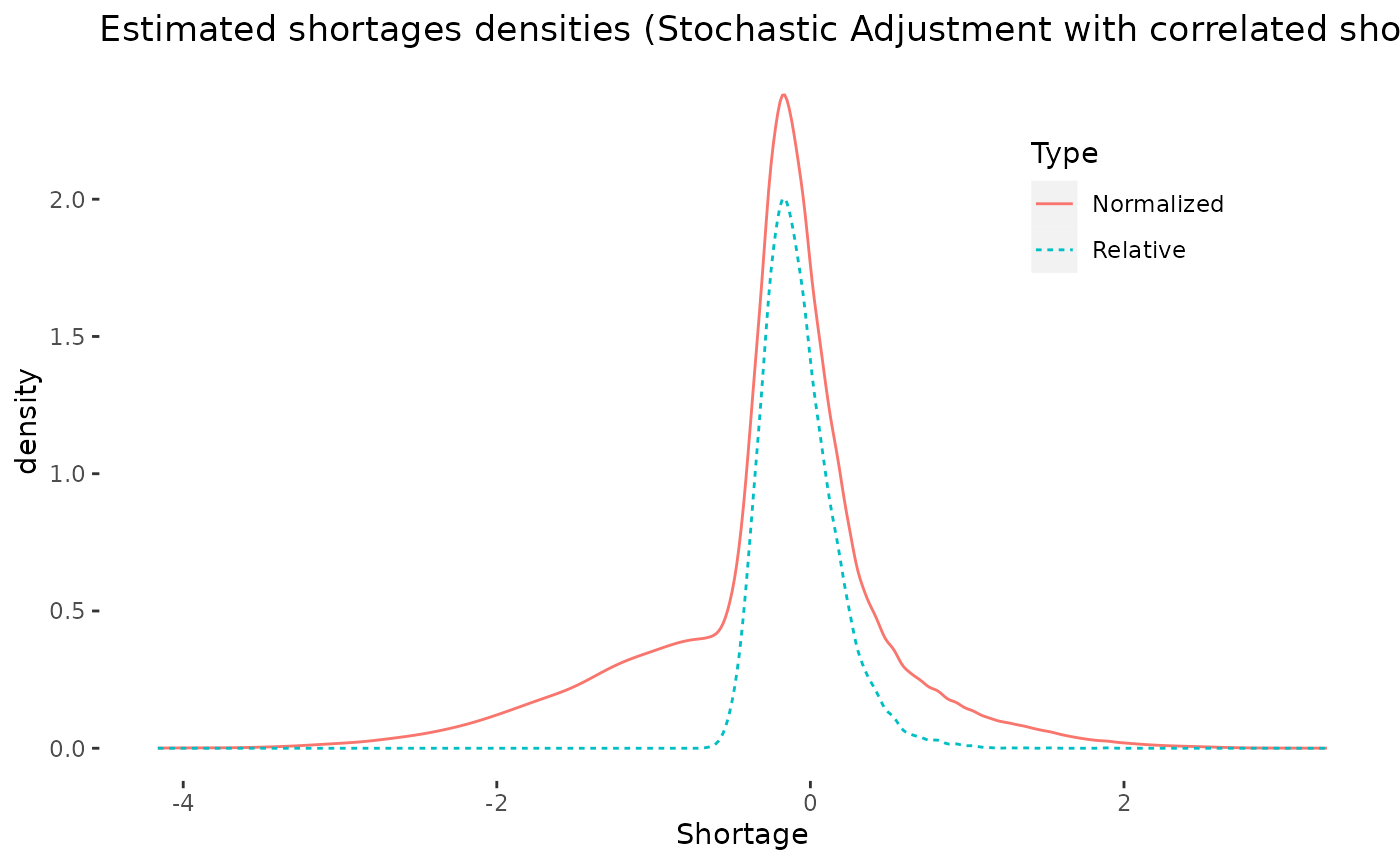
Copy the disequilibrium model tibble and augment it with post-estimation data. The disequilibrium models can be used to estimate:
Shortage probabilities. These are the probabilities that the disequilibrium models assign to observing a particular extent of excess demand.
Normalized shortages. The point estimates of the shortages are normalized by the variance of the difference of demand and supply shocks.
Relative shortages: The point estimates of the shortages are normalized by the estimated supplied quantity.
fit <- sa_fit
mdt <- tibble::add_column(
  fit@model_tibble,
  shortage_indicators = c(shortage_indicators(fit)),
  normalized_shortages = c(normalized_shortages(fit)),
  shortage_probabilities = c(shortage_probabilities(fit)),
  relative_shortages = c(relative_shortages(fit))
)
How is the sample separated post-estimation? The indices of the observations for which the estimated demand is greater than the estimated supply are easily obtained.
if (requireNamespace("ggplot2", quietly = TRUE)) {
  pdt <- tibble::tibble(
    Shortage = c(mdt$normalized_shortages, mdt$relative_shortages),
    Type = c(rep("Normalized", nrow(mdt)), rep("Relative", nrow(mdt))),
    xpos = c(rep(-1.0, nrow(mdt)), rep(1.0, nrow(mdt))),
    ypos = c(
      rep(0.8 * max(mdt$normalized_shortages), nrow(mdt)),
      rep(0.8 * max(mdt$relative_shortages), nrow(mdt))
    )
  )
  ggplot2::ggplot(pdt) +
    ggplot2::stat_density(ggplot2::aes(Shortage,
      linetype = Type,
      color = Type
    ), geom = "line") +
    ggplot2::ggtitle(paste0("Estimated shortages densities (", model_name(fit), ")")) +
    ggplot2::theme(
      panel.background = ggplot2::element_rect(fill = "transparent"),
      plot.background = ggplot2::element_rect(
        fill = "transparent",
        color = NA
      ),
      legend.background = ggplot2::element_rect(fill = "transparent"),
      legend.box.background = ggplot2::element_rect(
        fill = "transparent",
        color = NA
      ),
      legend.position = c(0.8, 0.8)
    )
} else {
    summary(mdt[, grep("shortage", colnames(mdt))])
}
Fitted values and aggregation
The estimated demanded and supplied quantities can be calculated per observation.
market <- cbind(
demand = demanded_quantities(fit)[, 1],
supply = supplied_quantities(fit)[, 1]
)
summary(market)
#> demand supply
#> Min. :3.175 Min. : 2.529
#> 1st Qu.:5.241 1st Qu.: 5.670
#> Median :5.684 Median : 6.366
#> Mean :5.683 Mean : 6.362
#> 3rd Qu.:6.129 3rd Qu.: 7.054
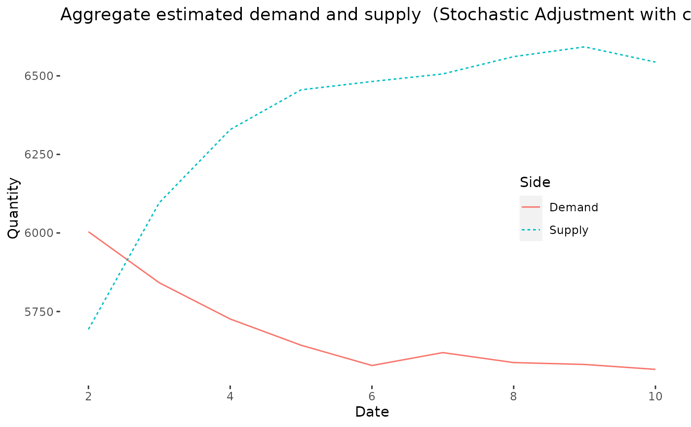
#> Max. :8.148 Max. :10.747The package also offers basic aggregation functionality.
aggregates <- aggregate_demand(fit) %>%
  dplyr::left_join(aggregate_supply(fit), by = "date") %>%
  dplyr::mutate(date = as.numeric(date)) %>%
  dplyr::rename(demand = D_Q, supply = S_Q)
if (requireNamespace("ggplot2", quietly = TRUE)) {
  pdt <- tibble::tibble(
    Date = c(aggregates$date, aggregates$date),
    Quantity = c(aggregates$demand, aggregates$supply),
    Side = c(rep("Demand", nrow(aggregates)), rep("Supply", nrow(aggregates)))
  )
  ggplot2::ggplot(pdt, ggplot2::aes(x = Date)) +
    ggplot2::geom_line(ggplot2::aes(y = Quantity, linetype = Side, color = Side)) +
    ggplot2::ggtitle(paste0(
      "Aggregate estimated demand and supply  (", model_name(fit), ")"
    )) +
    ggplot2::theme(
      panel.background = ggplot2::element_rect(fill = "transparent"),
      plot.background = ggplot2::element_rect(
        fill = "transparent", color = NA
      ),
      legend.background = ggplot2::element_rect(fill = "transparent"),
      legend.box.background = ggplot2::element_rect(
        fill = "transparent", color = NA
      ),
      legend.position = c(0.8, 0.5)
    )
} else {

    aggregates
}